The objective of this module is to introduce students to the fundamental principles of quantum computing.
The module covers the core concepts of qubits and quantum states, with emphasis on the phenomena of quantum superposition,
entanglement, decoherence, and quantum measurement, and their implications for information processing.
The foundational postulates of quantum mechanics underlying quantum computing are analyzed to provide a rigorous theoretical framework for these concepts.
Students will explore quantum gates and quantum circuits as the building blocks of quantum algorithms.
Practical implementation of these concepts will be demonstrated using a Python-based quantum computing library, enabling hands-on experience in designing and simulating quantum circuits.
Real-world applications of quantum computing will be illustrated through example exercises, including quantum cryptography,
to highlight the advantages and challenges of quantum approaches to secure communication.
Quantum computing is a multidisciplinary field comprising aspects of computer science, physics, and mathematics that aims to solve certain classes of complex problems faster and more efficiently than classical computers by exploiting quantum-mechanical principles.
[+]
Postulates of Quantum Mechanics for Information Processing
The postulates of quantum mechanics are fundamental principles that define how information can be represented,
manipulated, and measured within the quantum computing model.
Postulate 1: State Space
Associated with any isolated quantum system is a complex vector space with an inner product (a Hilbert space),
called the state space of the system. The system is completely described by its state vector \(|\psi \rangle \),
which is a unit vector in this space.
- Represents qubits and their superpositions
- Describes initialization of quantum registers
Postulate 2: Time Evolution
The evolution of a closed quantum system from time \(t_0\) to \(t_1\) is described by the unitary transformation:
$$
|\psi(t_1)\rangle = U |\psi(t_0)\rangle, \quad U^\dagger U = I
$$
- Quantum gates correspond to unitary operators
- The state \(|\psi \rangle \) changes via quantum gates
- All quantum algorithms are sequences of unitary operations (quantum circuits)
- Ensures reversibility of quantum computation
Postulate 3: Measurement
Quantum measurements are described by a collection of
measurement operators \(\{ M_m \}\), acting on the state space of the system. Each operator corresponds to a possible measurement outcome \(m\).
If the system is in the state \(|\psi \rangle \) immediately before the measurement, the probability of obtaining outcome \(m\) is
\(
p(m) = \langle \psi | M_m^\dagger M_m | \psi \rangle.
\)
The state of the system after measurement becomes
The state of the system after measurement becomes
$$
| \psi \rangle \xrightarrow{\text{Measurement}} \frac{M_m |\psi \rangle}{\sqrt{{\langle\psi|} M_m^\dagger M_m |\psi \rangle}}.
$$
The measurement operators satisfy the completeness relation
\(
\sum_m M_m^\dagger M_m = I,
\)
which ensures that the probabilities of all possible outcomes sum to one:
$$
\sum_m p(m) = \sum_m \langle \psi | M_m^\dagger M_m | \psi \rangle = 1 .
$$
- Explains probabilistic outcomes and collapse of superpositions
- Converts qubit superpositions into classical bits for readout
- Determines the output of quantum algorithms
- Implements projective measurements in quantum circuits
Postulate 4: Composition
The state space of a composite physical system is the tensor product of the state spaces of its subsystems.
If subsystem \(i\) is prepared in the state \(|\psi_i\rangle\), the joint state of the total system is
\( |\psi_1\rangle \otimes | \psi_2 \rangle \otimes ... \otimes |\psi_n\rangle\).
- Describes multi-qubit systems and entanglement
- Allows operations on subsystems or individual qubits
- Fundamental for quantum circuits, quantum teleportation, and entanglement-based algorithms
[+]
Fundamental Concepts of Quantum Computing
Qubits (quantum bits) are the basic units of quantum information, analogous to bits in classical computing.
While a classical bit can exist in only one of two states, \(0\) or \(1\), a qubit can exist in a superposition of the basis states \(|0 \rangle\) or \(|1 \rangle\):
Together, these properties give rise to quantum parallelism, in which a quantum computer evolves many computational paths simultaneously at the level of quantum state evolution. This enables certain problems to be solved more efficiently by reducing the number of computational steps and providing significant speedups for specific tasks such as search, factoring, and quantum simulation compared to classical approaches.
\begin{aligned}
\hspace{5em}
|\psi\rangle = \alpha |0\rangle + \beta |1\rangle \hspace{5em} \hfill (1)
\end{aligned}
where \(\alpha, \beta \in \mathbb{C}\) are complex amplitudes. The quantities \(|\alpha|^2\) and \(|\beta|^2\) represent the probabilities of measuring the states \(|0 \rangle\) and \(|1 \rangle\), respectively. The normalization condition ensures that the total probability is 1:
$$
|\alpha|^2 + |\beta|^2 = 1.
$$
\(\theta\):
\(\phi\):
α = 1, β = 0
- Eq.(1) is written in Dirac (bra–ket) notation, used in theory and quantum algorithms.
- The same physical qubit state, in column-vector (matrix) representation, is useful for computation and simulations:
$$ |\psi \rangle = \begin{bmatrix} \alpha \\ \beta \end{bmatrix}, \quad |0 \rangle \equiv \begin{bmatrix} 1 \\ 0 \end{bmatrix}, \quad |1 \rangle \equiv \begin{bmatrix} 0 \\ 1 \end{bmatrix} $$
-
For geometric visualization use the Bloch sphere representation:
\begin{aligned} |\psi \rangle = \cos \frac{\theta}{2} |0 \rangle + e^{i \phi} \sin \frac{\theta}{2} |1 \rangle \hspace{1em} \hfill (2) \\ \end{aligned} $$ \alpha = \cos \frac{\theta}{2}, \quad \beta = e^{i \phi} \sin \frac{\theta}{2}, $$where \(\theta, \phi \in \mathbb{R}\) are the polar and azimuthal angles. For a single qubit, the global phase factor has no physically observable effect and can be omitted.
Qubits' key properties:
- Superposition: A qubit can exist in a combination of \(|0 \rangle\) and \(|1 \rangle \) simultaneously.
- Measurement: When measured, a qubit collapses to either \(0\) or \(1 \) with probabilities determined by its state.
- Entanglement: Qubits can be correlated with each other in ways that have no classical counterpart.
- Interference: Quantum states can reinforce or cancel each other, enabling powerful computational effects.
Together, these properties give rise to quantum parallelism, in which a quantum computer evolves many computational paths simultaneously at the level of quantum state evolution. This enables certain problems to be solved more efficiently by reducing the number of computational steps and providing significant speedups for specific tasks such as search, factoring, and quantum simulation compared to classical approaches.
[+]
Superposition
The principle of superposition allows a qubit to exist in a combination of its basis states, \(|0 \rangle\) and \(|1 \rangle \) (Eq.(1)).
For an \(n\)-qubit system, the state can be a superposition of all \(2^n\) basis states:
Each \(|i\rangle\) represents a binary combination of the \(n\) qubits' basic states and can be expressed as a tensor product of the individual qubits:
For a two-qubit system (\(n = 2\)), there are four computational basis states: \(|00\rangle\), \(|01\rangle\), \(|10\rangle\), and \(|11\rangle\), where \(|01\rangle = |0\rangle \otimes |1\rangle,\) meaning the first qubit is \(|0\rangle\) and the second is \(|1\rangle\). The general state of a two-qubit system is a superposition of all four states:
In column-vector form:
To create superposition in a qubit, the Hadamard gate is widely used (see Quantum gates).
For an \(n\)-qubit system, the state can be a superposition of all \(2^n\) basis states:
\begin{aligned}
|\psi \rangle = \sum_{i=0}^{2^n-1} \alpha_i |i \rangle, \hspace{5em} \hfill (3)
\end{aligned}
where \(\alpha _i \in \mathbb{C}\) and \(\sum_{i=0}^{2^n-1} |\alpha _i |^2 = 1\).
Each \(|i\rangle\) represents a binary combination of the \(n\) qubits' basic states and can be expressed as a tensor product of the individual qubits:
$$
|q_1 q_2 \dots q_n \rangle = |q_1 \rangle \otimes |q_2 \rangle \otimes \dots \otimes|q_n \rangle ,
$$
where \(q_1, q_2, \dots, q_n\) denote the states of qubits 1 through \(n\), ordered left to right.
For a two-qubit system (\(n = 2\)), there are four computational basis states: \(|00\rangle\), \(|01\rangle\), \(|10\rangle\), and \(|11\rangle\), where \(|01\rangle = |0\rangle \otimes |1\rangle,\) meaning the first qubit is \(|0\rangle\) and the second is \(|1\rangle\). The general state of a two-qubit system is a superposition of all four states:
$$
|\psi\rangle = \alpha _0 |00\rangle + \alpha _1 |01\rangle + \alpha _2 |10\rangle + \alpha _3 |11\rangle,
$$
with \(\sum_{i=0}^{3} |\alpha _i |^2 = 1 \).
In column-vector form:
$$
|\psi\rangle
= \alpha_0
\begin{bmatrix}1\\0\\0\\0\end{bmatrix}
+ \alpha_1
\begin{bmatrix}0\\1\\0\\0\end{bmatrix}
+ \alpha_2
\begin{bmatrix}0\\0\\1\\0\end{bmatrix}
+ \alpha_3
\begin{bmatrix}0\\0\\0\\1\end{bmatrix}
=
\begin{bmatrix}
\alpha_0 \\
\alpha_1 \\
\alpha_2 \\
\alpha_3
\end{bmatrix}.
$$
To create superposition in a qubit, the Hadamard gate is widely used (see Quantum gates).
[+]
Mesurements
In quantum mechanics concept of measurement plays a crucial role in determining the outcome of a quantum experiment .
If the measurement operator \(M_m\) is projector onto the eigenstate \(|\phi_m \rangle\):
$$
M_m = | \phi_m \rangle \langle \phi_m |,
$$
the probability of observing that outcome is given by the Born rule:
\begin{aligned}
p(m) = \langle \psi | M_m |\psi \rangle = \langle \psi | \phi_m \rangle \langle \phi_m |\psi \rangle = |\langle \phi_m |\psi \rangle|^2 . \hspace{1em} \hfill (4)
\end{aligned}
After the measurement, the quantum state collapses to the observed eigenstate \(|\phi_m \rangle\):
$$
| \psi \rangle \xrightarrow{\text{measure m}} \frac{M_m | \psi \rangle}{\sqrt{p(m)}} = |\phi_m \rangle.
$$
Measurement in Quantum Computing
- Probabilistic nature: Measurement is inherently probabilistic. The probabilities of different outcomes are determined by the amplitudes of the quantum state according to the Born rule.
- State collapse: During measurement, the system transitions from a superposition to a definite state, turning the qubit into a classical bit. This phenomenon, known as wavefunction collapse, is a fundamental concept in quantum mechanics.
- Irreversibility: Measurement is irreversible — performing a measurement destroys information about the original superposition, which cannot be recovered.
- Partial measurements: Measuring one qubit can influence correlated qubits due to entanglement (Postulate 4, composition).
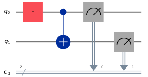
- Multiple runs: Because outcomes are probabilistic, quantum computers typically run the same circuit multiple times (called shots) to estimate the distribution of results. The final result is a statistical distribution of outcomes, not a single deterministic value.
[+]
Entanglement
Quantum entanglement is a fundamental property of quantum systems in which two or more qubits become correlated
in such a way that the state of one qubit cannot be described independently of the state of the others,
even when separated by large distances. This is a uniquely quantum-mechanical phenomenon that has no classical equivalent.
For two arbitrary quantum systems \(A\) and \(B\), with respective Hilbert spaces \(H_A\) and \(H_B\), a pure state is entangled if:
The canonical examples of maximally entangled two-qubit states, known as the Bell states, are:
Quantum entanglement is a key resource in quantum information processing. It underlies quantum teleportation, secure quantum communication, quantum error correction, and provides a fundamental advantage in many quantum algorithms.
For two arbitrary quantum systems \(A\) and \(B\), with respective Hilbert spaces \(H_A\) and \(H_B\), a pure state is entangled if:
-
It cannot be written as a tensor product of individual qubit states:
$$ |\psi \rangle \neq |\psi_A\rangle \otimes |\psi_B\rangle $$
-
Equivalently, the reduced density matrix of at least one subsystem is mixed:
$$ \text{Tr}(\rho_A^2) < 1 , \quad \text{or} \quad \text{Tr}(\rho_B^2) < 1 $$
The canonical examples of maximally entangled two-qubit states, known as the Bell states, are:
$$ |\Phi^\pm \rangle = \frac{|00\rangle \pm |11\rangle}{\sqrt{2}}, $$
$$ |\Psi^\pm \rangle = \frac{|01\rangle \pm |10\rangle}{\sqrt{2}}, $$
For the \(|\Psi^+\rangle\) Bell state, the joint measurement yields either \(|01\rangle\) or \(|10\rangle\) with equal probability,
but if the first qubit is found in state \(|0\rangle\), the second qubit is always found in \(|1\rangle\), and vice versa.
Thus, measurement causes the collapse of the joint quantum state.
Quantum entanglement is a key resource in quantum information processing. It underlies quantum teleportation, secure quantum communication, quantum error correction, and provides a fundamental advantage in many quantum algorithms.
[+]
Quantum gates
Quantum gates are reversible, unitary, and linear operations
that manipulate qubits and serve as the fundamental building blocks of quantum circuits,
analogous to how classical logic gates manipulate classical bits in digital circuits.
The properties of quantum gates are defined by the postulates of quantum mechanics (Postulate 2).
The output state can be obtained by applying a unitary matrix \(U\) to the initial state: $$ |\psi'\rangle = U |\psi\rangle $$ where \(U^\dagger U = U U^\dagger = I\), and \(U^\dagger\) denotes the conjugate transpose of \(U\). This ensures reversibility and conservation of probability.
Choose a quantum gate to see its matrix representation and learn how it affects qubits. Both single-qubit and multi-qubit (marked with *) gates are presented.
×
The identity gate is the identity matrix - square matrix with ones on the main diagonal and zeros elsewhere.
Leaves the qubit unchanged:
\(I|0\rangle = |0\rangle\)
\(I|1\rangle = |1\rangle \)
\(I|0\rangle = |0\rangle\)
\(I|1\rangle = |1\rangle \)
$$ I = \begin{pmatrix}1 & 0 \\0 & 1\end{pmatrix} $$
×
The Pauli gates \((X,Y,Z)\) are the three Pauli matrices \((\sigma _{x},\sigma _{y},\sigma _{z})\) that act on a single qubit.
The Pauli X, Y and Z equate, to a rotation around the \(x\), \(y\) and \(z\) axes of the Bloch sphere by \(\pi\) radians, respectively.
The Pauli X, Y and Z equate, to a rotation around the \(x\), \(y\) and \(z\) axes of the Bloch sphere by \(\pi\) radians, respectively.
Pauli-X (NOT) similar to the classical NOT gate,
Flips computational basis states:
\( X|{0}\rangle = |{1}\rangle \)
\( X|{1}\rangle = |{0}\rangle \)
Flips computational basis states:
\( X|{0}\rangle = |{1}\rangle \)
\( X|{1}\rangle = |{0}\rangle \)
$$X = \sigma_{x} = \begin{pmatrix}0 & 1 \\1 & 0\end{pmatrix} $$
Pauli-Y flips the computational basis states,
Adds a relative phase of \( \pm i \):
\( Y|{0}\rangle = i|{1}\rangle \)
\( Y|{1}\rangle = -i|{0}\rangle\)
Adds a relative phase of \( \pm i \):
\( Y|{0}\rangle = i|{1}\rangle \)
\( Y|{1}\rangle = -i|{0}\rangle\)
$$Y = \sigma_{y} = \begin{pmatrix}0 & -i \\ i & 0\end{pmatrix} $$
Pauli-Z leaves \(|0\rangle\) unchanged,
Adds a relative phase of \(\varphi = \pi\) to \(|1\rangle\):
\( Z|{0}\rangle = |{0}\rangle \)
\( Z|{1}\rangle = -|{1}\rangle \)
Adds a relative phase of \(\varphi = \pi\) to \(|1\rangle\):
\( Z|{0}\rangle = |{0}\rangle \)
\( Z|{1}\rangle = -|{1}\rangle \)
$$Z = \sigma_{z} = \begin{pmatrix}1 & 0 \\0 & -1\end{pmatrix} $$
×
The Hadamard gate is one of the most important single-qubit gates
used to create superpositions and enable parallelism in quantum computations.
When applied to a qubit initialized in a classical state \(|0\rangle\) or \(|1\rangle\),
the Hadamard gate transforms it into an equal superposition of both states,
making it a fundamental tool in quantum circuits.
It converts the computational (Z) basis \({|0\rangle, |1\rangle} \) into the X-basis \({|+\rangle, |-\rangle} \). Up to a global phase, this corresponds to a \(\pi\)-rotation around the \( (\hat{x} + \hat{z})/\sqrt{2}\) axis on the Bloch sphere.
It converts the computational (Z) basis \({|0\rangle, |1\rangle} \) into the X-basis \({|+\rangle, |-\rangle} \). Up to a global phase, this corresponds to a \(\pi\)-rotation around the \( (\hat{x} + \hat{z})/\sqrt{2}\) axis on the Bloch sphere.
\( H|{0}\rangle = \frac{|{0}\rangle + |{1}\rangle}{\sqrt{2}} = |+\rangle \)
\(H|{1}\rangle = \frac{|{0}\rangle - |{1}\rangle}{\sqrt{2}} = |-\rangle\)
\(H|{1}\rangle = \frac{|{0}\rangle - |{1}\rangle}{\sqrt{2}} = |-\rangle\)
$$ H = \frac{1}{\sqrt{2}}\begin{pmatrix}1 & 1 \\1 & -1\end{pmatrix} $$
×
The phase shift is a family of single-qubit gates that map the basis states
\( |0\rangle \mapsto |0\rangle \) and \(|1\rangle \mapsto e^{i\varphi }|1\rangle \).
Applying the gate modifies the phase of the quantum state. This is equivalent to a rotation about
the \(z\)-axis on the Bloch sphere by \(\varphi\) radians.
The phase shift gates are represented by the matrix (\(P^{\dagger }(\varphi )=P(-\varphi )\)):
$$ P(\varphi )={\begin{pmatrix}1&0\\0&e^{i\varphi }\end{pmatrix}}$$
where \(\varphi\) is the phase shift with the \(2\pi\) period.
Leaves \(|0\rangle\) unchanged and adds a relative phase of \(\varphi = \pi/2\) to \(|1\rangle\):
Leaves \(|0\rangle\) unchanged and adds a relative phase of \(\varphi = \pi/2\) to \(|1\rangle\):
\( S|0\rangle = |0\rangle \)
\( S|1\rangle = i|1\rangle \)
\( S|1\rangle = i|1\rangle \)
$$ S = \begin{pmatrix}1 & 0 \\0 & i\end{pmatrix} $$
×
The phase shift is a family of single-qubit gates that map the basis states
\( |0\rangle \mapsto |0\rangle \) and \(|1\rangle \mapsto e^{i\varphi }|1\rangle \).
Applying the gate modifies the phase of the quantum state. This is equivalent to a rotation about
the \(z\)-axis on the Bloch sphere by \(\varphi\) radians.
The phase shift gates are represented by the matrix (\(P^{\dagger }(\varphi )=P(-\varphi )\)):
$$ P(\varphi )={\begin{pmatrix}1&0\\0&e^{i\varphi }\end{pmatrix}}$$
where \(\varphi\) is the phase shift with the \(2\pi\) period.
Leaves \(|0\rangle\) unchanged and adds a relative phase of \(\varphi = \pi/4\) to \(|1\rangle\):
Leaves \(|0\rangle\) unchanged and adds a relative phase of \(\varphi = \pi/4\) to \(|1\rangle\):
\( T|0\rangle = |0\rangle \)
\( T|1\rangle = e^{i\pi/4}|1\rangle \)
\( T|1\rangle = e^{i\pi/4}|1\rangle \)
$$ T = \begin{pmatrix}1 & 0 \\0 & e^{i\pi/4}\end{pmatrix} $$
×
Controlled-NOT (CNOT or controlled Pauli-X) is a two-qubit gate. The second (target) qubit is flipped only
if the first (control) qubit is \(|1\rangle\).
$$
|00\rangle \rightarrow |00\rangle,\quad
|01\rangle \rightarrow |01\rangle,\quad
|10\rangle \rightarrow |11\rangle,\quad
|11\rangle \rightarrow |10\rangle
$$
$$ \text{CNOT} =\begin{pmatrix}1&0&0&0\\0&1&0&0\\0&0&0&1\\0&0&1&0\end{pmatrix} $$
×
Controlled-Z (CZ) is a two-qubit gate. It applies a phase flip only when both qubits are in the state \(|1\rangle\).
$$ |00\rangle \rightarrow |00\rangle,\quad |01\rangle \rightarrow |01\rangle,\quad |10\rangle \rightarrow |10\rangle,\quad |11\rangle \rightarrow -|11\rangle $$
$$ |00\rangle \rightarrow |00\rangle,\quad |01\rangle \rightarrow |01\rangle,\quad |10\rangle \rightarrow |10\rangle,\quad |11\rangle \rightarrow -|11\rangle $$
$$ \text{CZ} = \begin{pmatrix}1&0&0&0\\0&1&0&0\\0&0&1&0\\0&0&0&-1\end{pmatrix} $$
The controlled-Z gate is the special case of the controlled-U gate, with U = Z.
More generally, a controlled-U gate applies an arbitrary single-qubit operator U to the target qubit
when the control qubit is \(|1\rangle\). Choosing U = X, Y or Z yields the controlled-X (CNOT), controlled-Y, and controlled-Z gates, respectively.
$$ \text{U} =\begin{pmatrix}1&0&0&0\\0&1&0&0\\0&0&u_{00}&u_{01}\\0&0&u_{10}&u_{11}\end{pmatrix} $$
×
The SWAP gate swaps the states of two qubits. With respect to the basis \(|00\rangle \),
\(|01\rangle \), \(|10\rangle \), \(|11\rangle \), it is represented by the matrix:
$$ \text{SWAP} = \begin{pmatrix}1&0&0&0\\0&0&1&0\\0&1&0&0\\0&0&0&1\end{pmatrix} $$
×
The Toffoli gate (CCNOT) is defined for 3 qubits. If we limit ourselves to only accepting input qubits
that are \( |0\rangle \) and \(|1\rangle \), then if the first two bits are in the state \(|1\rangle \)
it applies a Pauli-X (or NOT) on the third bit.
$$ \text{CCNOT} = \begin{pmatrix}1&0&0&0&0&0&0&0\\0&1&0&0&0&0&0&0\\0&0&1&0&0&0&0&0\\0&0&0&1&0&0&0&0\\0&0&0&0&1&0&0&0\\0&0&0&0&0&1&0&0\\0&0&0&0&0&0&0&1\\0&0&0&0&0&0&1&0\end{pmatrix}$$
[+]
Application: VQE algoritm for eigenvalue problems
The variational quantum eigensolver (VQE)
is a hybrid quantum–classical algorithm that employs a variational principle to find approximate solutions
to optimization and quantum simulation problems.
In VQE, the goal is to approximate the ground-state energy of a quantum system described by a qubit Hamiltonian by adjusting variational parameters \(\theta\),
where the minimum eigenvalue corresponds to the ground-state energy of the quantum system:
$$
min_{\theta}\langle\psi(\theta_i)|H_\text{qubit}|\psi(\theta_i)\rangle.
$$
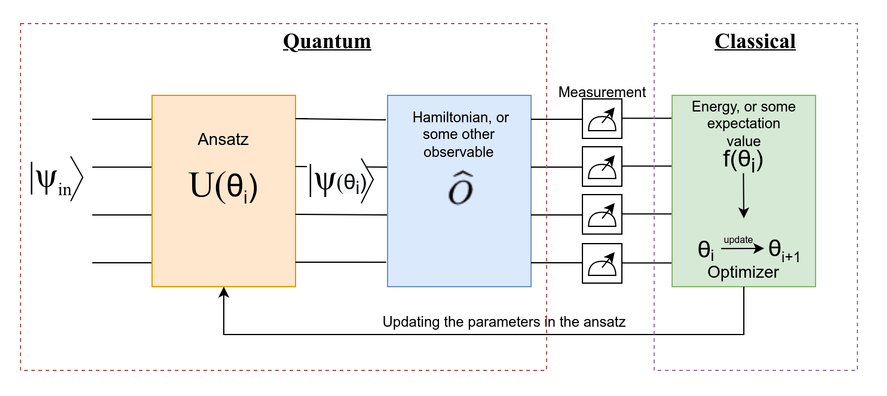
VQE is primarily used in quantum chemistry and materials science to estimate the ground-state energies of molecular and solid-state systems and provides a promising alternative by combining quantum resources with classical optimization, enabling efficient exploration of complex quantum systems.
The algorithm begins by preparing an initial quantum state \( | \psi \rangle \),
which is typically chosen as the computational basis state \( | 0 \rangle \).
A parameterized quantum circuit, known as the ansatz \( U(\theta)\) is then applied to generate a trial quantum state \(|\psi \rangle\).
Measurements of this state are performed to estimate the expectation value of the Hamiltonian, which serves as the objective observable.
A classical optimizer iteratively updates the variational parameters based on the measurement outcomes, seeking to minimize the energy expectation value.
This quantum-classical feedback loop is repeated until convergence is reached.
The resulting energy provides an approximation to the ground-state energy of the system.
The Variational Quantum Eigensolver (VQE) algorithm
is employed to compute the ground-state energy of the hydrogen molecule (\(H_2\)) at various internuclear distances using
Qiskit (v2.3.0), a Python-based quantum computing framework developed by IBM .
[+]
Complete Procedure to Compute the Ground-State Energy of H₂ Using VQE
Step 0:
Physical system H\(_2\)
Physical system H\(_2\)
Electronic Hamiltonian (Born-Oppenheimer approximation):
$$
H = -\frac12 \nabla_1^2 - \frac12 \nabla_2^2 - \frac{1}{r_{1A}} - \frac{1}{r_{1B}} - \frac{1}{r_{2A}} - \frac{1}{r_{2B}} + \frac{1}{r_{12}}
$$
Step 1:
Atomic basis set
Atomic basis set
Minimal basis sto-3g: for the H₂ molecule - one 1s orbital per hydrogen atom.
$$
\phi_A(\mathbf r) = \sum_{k=1}^3 d_k e^{-\alpha_k |\mathbf r - \mathbf R_A|^2}, \quad
\phi_B(\mathbf r) = \sum_{k=1}^3 d_k e^{-\alpha_k |\mathbf r - \mathbf R_B|^2}
$$
Normalization: \(\int |\phi_A|^2 d^3r = \int |\phi_B|^2 d^3 r = 1\)
Step 2:
Spin-orbitals
Spin-orbitals
Each spin-orbital represents a quantum state of an electron:
$$ |\chi\rangle = |\phi\rangle \otimes |\sigma\rangle $$
where \(|\phi\rangle\) is a spatial orbital, \(|\sigma\rangle\) is a spin state: \(\alpha\) - spin up and \(\beta\) - spin down.
For \(\text{H}_2\), we define four spin-orbitals:
$$
\chi_0 = \phi_A \alpha, \quad
\chi_1 = \phi_A \beta , \quad
\chi_2 = \phi_B \alpha, \quad
\chi_3 = \phi_B \beta
$$
To use a quantum computer, we introduce occupation number encoding:
- \(|0\rangle\) - empty spin-orbital (no electron)
- \(|1\rangle\) - occupied spin-orbital (one electron)
Step 3:
Calculation of integrals
Calculation of integrals
One-electron integrals:
\(
h_{pq} = \langle \chi_p | -\frac12 \nabla^2 - \frac{1}{r_{1A}} - \frac{1}{r_{1B}} | \chi_q \rangle
\)
Two-electron integrals: \( g_{pqrs} = \langle \chi_p \chi_q | \frac{1}{r_{12}} | \chi_r \chi_s \rangle \)
Two-electron integrals: \( g_{pqrs} = \langle \chi_p \chi_q | \frac{1}{r_{12}} | \chi_r \chi_s \rangle \)
Step 4:
Fermionic Hamiltonian
Fermionic Hamiltonian
$$
H = \sum_{pq} h_{pq} a_p^\dagger a_q + \frac12 \sum_{pqrs} g_{pqrs} a_p^\dagger a_q^\dagger a_r a_s
$$
Step 5:
Fermion - to - qubit
transformation
Fermion - to - qubit
transformation
The fermionic Hamiltonian (Step 4) is mapped to qubits Hamiltonian using transformation of Jordan-Wigner:
$$
a_j = \left( \prod_{k=0}^{j-1} Z_k \right)\frac{X_j + iY_j}{2}
$$
$$
a_j^\dagger = \left( \prod_{k=0}^{j-1} Z_k \right)\frac{X_j - iY_j}{2}
$$
One spin orbital corresponds to one qubit: 4 spin-orbitals → 4 qubits:
$$
a_0 = \frac{X_0 + i Y_0}{2}, \quad a_0^\dagger = \frac{X_0 - i Y_0}{2}
$$
$$
a_1 = Z_0 \frac{X_1 + i Y_1}{2}, \quad a_1^\dagger = Z_0 \frac{X_1 - i Y_1}{2}
$$
$$
a_2 = Z_0Z_1 \frac{X_2 + i Y_2}{2}, \quad a_2^\dagger= Z_0Z_1 \frac{X_2 - i Y_2}{2}
$$
$$
a_3 = Z_0Z_1Z_2 \frac{X_3 + i Y_3}{2}, \quad a_3^\dagger = Z_0Z_1Z_2 \frac{X_3 - i Y_3}{2}
$$
The operator \( n_j = a_j^\dagger a_j \) determines the occupation of spin-orbital \( j \), giving 1 if it is occupied and 0 if it is empty.
Substituting the Jordan-Wigner transformation of the fermionic operators \( a_j^\dagger \) and \( a_j \) leads to
$$
n_j = a_j^\dagger a_j = \frac{1-Z_j}{2},
$$
which connects fermionic occupation with qubit Pauli operators.
Step 6:
Final qubit Hamiltonian
Final qubit Hamiltonian
After applying the Jordan-Wigner transformation, the fermionic Hamiltonian is mapped to a 4-qubit Hamiltonian
expressed as a sum of Pauli strings:
$$
H_q = c_0 I + c_1 Z_0 + c_2 Z_1 + c_3 Z_2 + c_4 Z_3 \\
+ c_5 Z_0 Z_1 + c_6 Z_0 Z_2 + c_7 Z_0 Z_3
+ c_8 Z_1 Z_2 + c_9 Z_1 Z_3 + c_{10} Z_2 Z_3 \\
+ c_{11} \big(
X_0 Y_1 Y_2 X_3
- X_0 X_1 Y_2 Y_3
- Y_0 Y_1 X_2 X_3
+ Y_0 X_1 X_2 Y_3\big)
$$
The coefficients \(c_i\) are functions of the one-electron integrals \(h_{pq}\) and two-electron integrals \(g_{pqrs}\) calculated in Step 3.
Step 7:
Reduction by singlet symmetry
Reduction by singlet symmetry
For 2 electrons in 4 spin orbitals → 6 determinants
$$ |1100\rangle, |1010\rangle, |1001\rangle, |0110\rangle, |0101\rangle, |0011\rangle $$
Each bitstring indicates the occupation of spin-orbitals in the order ($\chi_0, \chi_1, \chi_2, \chi_3$): 1 - occupied, 0 - unoccupied.
These states can be classified according to total spin:
Each bitstring indicates the occupation of spin-orbitals in the order ($\chi_0, \chi_1, \chi_2, \chi_3$): 1 - occupied, 0 - unoccupied.
These states can be classified according to total spin:
- Singlets (S = 0): \( |1100\rangle, |0011\rangle, \frac{|1001\rangle - |0110\rangle}{\sqrt{2}} \) → the ground state of H\(_2\) is a singlet;
- Triplets (S = 1): \( |1010\rangle, |0101\rangle, \frac{|1001\rangle + |0110\rangle}{\sqrt{2}} \) → do not contribute to the ground state.
Step 8:
Construction of logical qubits
Construction of logical qubits
Due to additional spatial symmetry (particle number + spin symmetry + spatial symmetry),
the ground state can be well approximated within the 2-dimensional subspace.
For the reduced ground-state model, the best basis is
$$
|1100\rangle, |0011\rangle.
$$
Logical basis is defined as:
$$
|0\rangle_\text{logical} \equiv |1100 \rangle , \quad
|1\rangle_\text{logical} \equiv |0011\rangle
$$
In the molecular orbital basis, the states \(|1100 \rangle\) and \(|0011\rangle\) correspond to double occupation of the bonding and antibonding molecular orbitals, respectively.
Step 9:
Reduced Hamiltonian
Reduced Hamiltonian
After symmetry reduction (Step 7), the Hamiltonian (Step 6) projected onto a reduced 2-dimensional subspace in the reduced basis { \(|0\rangle_\text{logical}, |1\rangle_\text{logical}\) } can be expressed :
$$
H_{logical} = c_0 I + c_1 Z + c_2 X ,
$$
where
$$
c_0 = h_{00} + h_{11} + \frac{g_{0000} + g_{1111}}{2} \\
c_1 = h_{00} - h_{11} + \frac{ (g_{0000} - g_{1111}) }{2}, \\
c_2 = g_{0101}.
$$
The final qubit Hamiltonian depends on the choice of orbital basis, fermion-to-qubit mapping, and symmetry reductions applied during the mapping procedure. Different effective qubit representations (for example, 4-qubit, 2-qubit, or reduced 1-qubit models for \(\text{H}_2\)) lead to different Pauli-string forms of the Hamiltonian while describing the same physical system.
The final qubit Hamiltonian depends on the choice of orbital basis, fermion-to-qubit mapping, and symmetry reductions applied during the mapping procedure. Different effective qubit representations (for example, 4-qubit, 2-qubit, or reduced 1-qubit models for \(\text{H}_2\)) lead to different Pauli-string forms of the Hamiltonian while describing the same physical system.
Step 10:
VQE Ansatz
VQE Ansatz
Since the reduced space is 2-dimensional, the trial state can be written as
$$|\psi(\theta)\rangle = \cos\theta |0\rangle_\text{logical} - \sin\theta |1\rangle_\text{logical} $$
the parameter \(\theta\) is sufficient to span the entire singlet subspace.
Step 11:
VQE Procedure
VQE Procedure
- Prepare \(|\psi(\theta)\rangle\) on 1 qubit.
- Measure \(E(\theta) = \langle \psi(\theta)|H|\psi(\theta)\rangle\).
- Optimize \(\theta\) to minimize \(E(\theta)\).
- Result: The minimum value of \(E_\text{VQE} \approx E_\text{0}\) within the chosen basis.
1. Enter coordinates \(r_1\), \(r_2\) and the number of spatial points \(N\) between them:
\(r_1=\) Å,
\(r_2=\)Å,
\(N=\).
2. Building the physical model:
The molecular system is defined using PySCF - a Python-based quantum chemistry package that performs classical electronic structure calculations to generate the fermionic Hamiltonian [see Step 4].
The molecular system is defined using PySCF - a Python-based quantum chemistry package that performs classical electronic structure calculations to generate the fermionic Hamiltonian [see Step 4].
The atomic structure, charge, spin and basis set
must be defined for the hydrogen molecule \(H_2\) :
- charge = 0 - the system is assumed to be neutral
- spin = 0
- the basis set =
3. Hamiltonian Preparation :
The fermionic Hamiltonian of the molecular system is mapped to a qubit Hamiltonian
using a fermion-to-qubit transformation [see Step 7]:
→ can be expressed as a weighted sum of Pauli operators acting on qubits;
→ compatible with quantum circuit execution and measurement.
→ can be expressed as a weighted sum of Pauli operators acting on qubits;
→ compatible with quantum circuit execution and measurement.
$$
H_{\text{qubit}} = \sum_{i} c_i\, P_i, \quad P_i \in \{I, X, Y, Z\}^{\otimes n} ,
$$
where \(c_i\) are function of \(h_{pq}\) and \(g_{pqrs}\) [see Steps 5, 6].
4. Ansatz Preparation:
An ansatz is a parameterized quantum circuit that defines a family of trial quantum states,
from which the optimizer searches for the ground state of the Hamiltonian [see Step 8]:
$$
|\psi(\theta)\rangle = U(\theta)|\psi_{\text{in}}(\theta)\rangle.
$$
The choice of ansatz depends on the physical system being modeled and is critical for convergence of the algorithm.
5. Classical Optimization:
A classical optimizer iteratively updates the variational parameters
\(\theta\) to minimize the energy, forming a quantum-classical feedback loop.
You can select different optimizers from the dropdown menu: and clarified the maximum iterations in the optimazer: \(MAX_{iter}=\).
Select a point (\(E(r)\)) to plot its convergence during calculation: \(n = \)
You can select different optimizers from the dropdown menu: and clarified the maximum iterations in the optimazer: \(MAX_{iter}=\).
Select a point (\(E(r)\)) to plot its convergence during calculation: \(n = \)
6. Quantum Circuit Execution.
A statevector-based estimator is used, allowing exact evaluation of expectation values in a noiseless simulation. On real quantum hardware, these expectation values are estimated statistically from repeated circuit executions.
A statevector-based estimator is used, allowing exact evaluation of expectation values in a noiseless simulation. On real quantum hardware, these expectation values are estimated statistically from repeated circuit executions.
[+]
Visualization of the Ground-State Optimization Process
THE PROJECT IS SUPPORTED BY