Chapter 1 - Trace Gas Detection: Photoionization cross section

Objective: In this module, we will explore the fundamental process of the photoionization of atoms, a crucial technique in quantum technology for the creation, control, and manipulation of quantum systems. The module will focus on calculating the wave functions of an electron in both bound and free states as a result of photoionization and determining the photoionization cross-section for characterizing the process. By the end of the module, students will have a deep understanding of these core topics and their applications in quantum systems, preparing them for further studies in quantum mechanics and technology.

We consider the process of ionization of an atom. The origin of energy is chosen to be at the energy of ionization $E_{th}: E_{th}=0$. Therefore, the initial bound state $\vert i\rangle$ of the atom has a negative energy $E_i < E_{th}$, while after ionization, in the final state $\vert f\rangle$, when one of the electrons is at an infinite distance from the atom, the energy of the system is positive $E_f>E_{th}$.

For the simplicity of the discussion, it is assumed that only one electron in the outer electronic shell participates in the process. The assumption gives the exact result for one-electron systems (such as H or He$^+$). The assumption is a very good approximation for alkali atoms and for many situations of excited states of other atoms. However, the approximation is not accurate for such atoms as He or Ne in their ground electronic state.

It is also assumed that the $ z $-axis of the laboratory reference frame is chosen along the axis of polarization of the incident light. In this situation, the photoionization (PI) cross section is given by the formula

$$\sigma^{PI}=\frac{4\pi^2 e^2}{c}\omega \left| \hat z_{fi} \right|^2\,,$$

where $\hat z$ is the $ z $-coordinate of the active electron. In the general case, a sum over the $ z $ components of all electrons should be evaluated.

In the above expression $\vert i\rangle$ and $\vert f\rangle$ are initial and final states of the system. Because one-electron approximation is used, the wave functions of $\vert i\rangle$ and $\vert f\rangle$ are written as

$$\vert i\rangle=R_i(r) Y_{l_i m_i}(\theta,\phi),$$ $$\vert f\rangle= R_f(r) Y_{l_f m_f}(\theta,\phi)$$

and the $ z $ component of the electron is represented by spherical coordinates

$$\hat z = r\cos(\theta)=\sqrt{\frac{4\pi}{3}}r Y_{1,0}(\theta,\phi),$$ $$ \hat z_{fi}=\langle R_f \vert r \vert R_i \rangle \sqrt{\frac{4\pi}{3}}\langle Y_{l_f m_f} \vert Y_{10} \vert Y_{l_i m_i} \rangle . $$

The angular part of the integral in the matrix element $\hat z_{fi}$ is evaluated analytically

$$ \langle Y_{l_f m_f} \vert Y_{10} \vert Y_{l_i m_i} \rangle =\sqrt{\frac{2l_i+1}{2l_f +1}} \sqrt{\frac{3}{4\pi}} C_{l_i 0 1 0}^{l_f 0}C_{l_i m_i 1 0}^{l_f m_f}\,. $$

Using the notation $r_{fi}=\langle R_f \vert r \vert R_i \rangle$, $\hat z_{fi}$ becomes

$$ \hat z_{fi}=r_{fi}\sqrt{\frac{2l_i+1}{2l_f+1}}C_{l_i 0 1 0}^{l_f 0}C_{l_i m_i 1 0}^{l_f m_i}\delta_{m_i m_f}\,. $$

The above derivation is made for a given initial state $\vert i\rangle$ of the atom and a given final state of $\vert f\rangle$ of the ion, and for a polarization of the electromagnetic field along $z$-axis in laboratory frame.

If the initial polarization is random and one is interested in the PI cross section into all possible polarizations of the final state, one should average the PI cross section over initial states and make a sum over final states, i.e.

$$ \frac{1}{2l_i+1}\sum_{m_i,m_f}\vert z_{fi} \vert^2=\frac{1}{3}\vert C_{l_i~0;1~0}^{l_f~0}\vert^2 \vert r_{fi}\vert^2 , $$ so that such a PI cross section averaged over polarizations is $$ \sigma^{PI}=\frac{4\pi^2 e^2}{3c}\omega \vert C_{l_i~0;1~0}^{l_f~0}\vert^2 \vert r_{fi}\vert^2\,, $$ without averaging over initial polarizations but summed over final polarizations is $$ \sigma^{PI}_{m_i}=\frac{4\pi^2 e^2}{c}\frac{2l_i+1}{2l_f +1}\omega \vert C_{l_i~m_i;1~0}^{l_f~m_i}\vert^2 \vert C_{l~0;1~0}^{l'~0}\vert^2 \vert r_{fi}\vert^2\,. $$

Radial functions $R_i=\frac{\chi_i}{r}$ and $R_f=\frac{\chi_f}{r}$ are obtained solving the radial Schrodinger equation

$$ -\frac{\hbar^2}{2m_e}\frac{d^2\chi}{dr^2}+\left(\frac{\hbar^2 l(l+1)}{2m_er^2} +V(r)\right)\chi=E\chi\, $$

for the corresponding ($E_i < 0$ and $E_f > 0$) energies. The potential of interaction is a pure Coulomb potential $V(r)=-\frac{Ze^2}{r}$ if the atom has only one electron, such as H, He$^+ $, etc. For multi-electron atoms, $V(r)$ behaves as $-\frac{Ze^2}{r}$ only for large distances $r$.

At large values of $r$, the bound-state wave function $\chi_i(r)\to 0$, while $\chi_f(r)$ oscillates. For pure Coulomn field, the asymptotic behavior of $\chi_f(r)$ is

$$\chi_f(r)\to \sqrt{\frac{2}{\pi k}}\sin(kr+\frac{\ln (r)}{k}+\sigma_C).$$

[+]

Coulomb functions for negative energies

[+]

Coulomb functions for positive energies

The regular Coulomb wave function can be computed by utilizing the mpmath library's coulombf$(l, \eta, z)$ function: $$ F_l(\eta,z) = C_l(\eta) z^{l+1} e^{-iz} \,_1F_1(l+1-i\eta, 2l+2, 2iz), $$ where the normalization constant $C_l(\eta)$ is as calculated by coulombc(). This function solves the differential equation $$f''(z) + \left(1-\frac{2\eta}{z}-\frac{l(l+1)}{z^2}\right) f(z) = 0.$$ A second linearly independent solution is given by the irregular Coulomb wave function $G_l(\eta,z)$ (see coulombg()). The Coulomb wave functions with real parameters are defined in "Abramowitz & Stegun", section 14. However, all parameters are permitted to be complex in this implementation (see references).

To solve the Schrodinger equation for the Coulomb potential $$ -\frac{\hbar^2}{2m_e}\frac{d^2\chi}{dr^2}+\left(-E+\frac{\hbar^2 l(l+1)}{2m_er^2}-\frac{Ze^2}{r}\right)\chi=0 $$ with $E>0$ we transforme it into a form where the Colomb functions (see above) can be applied. After the change $r=az$ and $\chi=bf$ is transformed to $$ \frac{\hbar^2 b}{2m_ea^2}\frac{d^2w}{dz^2}+\left(bE-\frac{\hbar^2 b l(l+1)}{2m_ea^2z^2}+\frac{Ze^2b}{az}\right)f=0 $$ with $bE=1$ ($b>0$) and $\frac{\hbar^2 b}{2m_ea^2}=1$ the equation is brought to the top one $$\frac{d^2f}{dz^2} - \left(1+\frac{Ze^2}{\hbar}\sqrt{\frac{2m_e}{E}}\frac{1}{z}- \frac{l(l+1)}{z^2}\right) w = 0$$ i.e. $\eta=-\frac{Ze^2}{\hbar}\sqrt{\frac{m_e}{2E}}.$ It has the same form as the effective quantum number but with positive $E$. The scaling factor $a$ for coordinate is $a=\frac{\hbar}{\sqrt{2m_eE}}.$

[+]

Photoionization cross section

[+]

Application: Photoionization Detector

One application of gas photoionization is the measurement of small concentrations (ranging from sub-parts per billion to 10,000 parts per million (ppm)) of volatile organic compounds (VOCs) and other gases using photoionization detectors (PIDs), as illustrated in Figure 1. PTL.

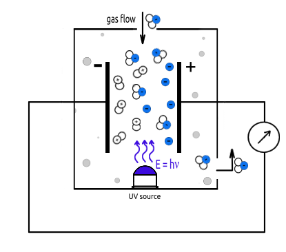
The PID is a portable, nonspecific, vapor/gas detector employing the principle of photoionization to detect a variety of chemical compounds, both organic and inorganic, in air.

The operation of a Photoionization Detector (PID) relies on measuring the current generated by the ionization of gases and vapors when exposed to photons emitted by an ultraviolet (UV) light source (1). The energy of these photons is typically falls between 8.4 eV and 11.7 eV, depending on the type of lamp used. These energy levels determine which compounds a PID can detect. The UV light source emits radiation into an ionization chamber (3) that contains two electrodes (2). One electrode is connected to a power source, and the other to an electrometer.

When a gas sample is introduced into the ionization chamber, components with ionization energies lower than the photon energy of the lamp are ionized (for example, a 10.6 eV lamp can detect compounds like benzene with ionization potential around 9.25 eV). This ionization process generates a current within the chamber, and the current's magnitude is directly proportional to the concentration of ionizable impurities in the sample. Notably, components of clean air, such as oxygen, nitrogen, argon, methane, carbon monoxide, and carbon dioxide, are not ionized under these conditions, as their ionization energies typically exceed 12.0 eV.

As a result, the PID is a highly efficient and cost-effective tool for monitoring potential worker exposure to VOCs, such as solvents, fuels, degreasers, plastics, and other compounds during manufacturing processes.

Advantages of PIDs are high sensitivity, fast response time, stability and durability, long service life. However, PIDs have limitations, such as non-selectivity and sensitivity to humidity. Despite these factors, PIDs remain highly effective as a rapid method for measuring VOC concentrations in air, within a wide temperature range of -30°C to 50°C.

Open notebook

v.1.2 [15.06.2023-15.07.2024]. Full-stack programming and site design by M. Sosnova (mariya.v.sosnova@gmail.com)

Whittaker functions